Sections
Geneious Prime
Geneious Prime is a molecular biology and sequence analysis tool, and helps you to organize data and projects in an efficient way.
Note
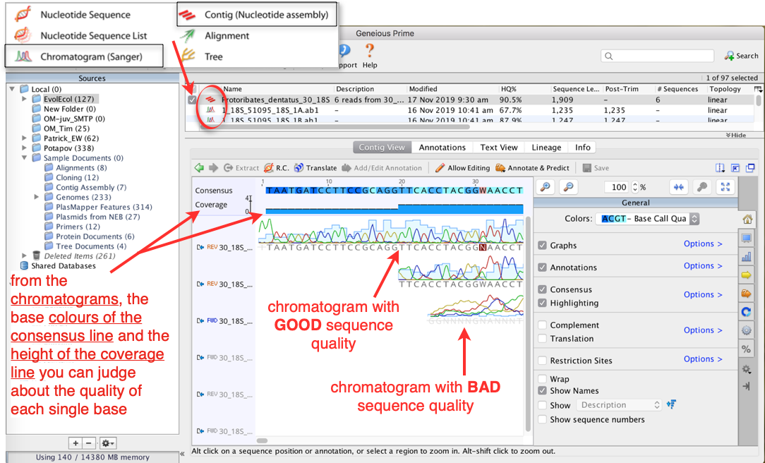
It is important that the consensus sequences are of high quality (checked for sequencing errors or true heterozygosity) and that ambiguous positions are removed in order to infer correct phylogenies. Standard Sanger sequencing methods produce DNA sequences of ~700-900 bp long, however ~30 bp at the start/end of the sequence is usally of poor quality. This is due to primer deterioration, incorrect primer annealing, and/or aborted elongation, as well as technical limitations in accurately separating very short and very long DNA strands at the nucleotide level. To obtain high quality consensus sequences, it is common to sequence and assemble the forward and reverse strands of a PCR product. In this way it is possible to correct ambigous positions. Furthermore, by assembling forward and reverse sequences, the resulting consensus sequence is usually longer than any single strand, thus providing more phylogenetic information. Sequencing facilities normally provide raw sequencing data in .abi format (also known as DNA trace file). This file contains the DNA sequence electropherogram as well as raw data. The electropherogram (=chromatogram) shows the DNA trace during the sequencing process and can be viewed graphically. Most sequencing editors can open .abi trace files, such as BioEdit. However, most sequencing editors and analyses software that combine the DNA sequence and the chromatogram in a single analysis window, which considerably simplifies the processing of sequences, are commercial (e.g. Sequencher, CodonCodeAligner). Geneious Prime (Biomatters) provides a 30-day trial version, which we will use for analysing the sequences generated last week. You can download Geneious Prime here and install it on your PC. If you want to watch a tutorial about Geneious Prime see here or under Lectures.
Working with Geneious Prime
Launch Geneious Prime
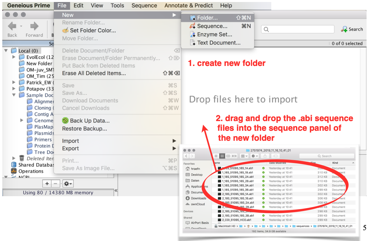
Create a new folder for your project
Drag and drop the
.abifiles from your explorer/finder into the sequence panel to import the sequence files
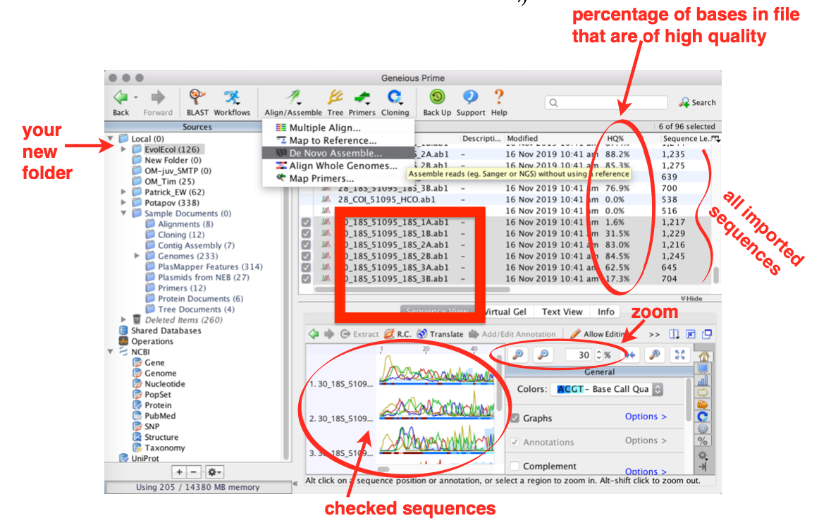
Check out all single sequence files that belong to the same sample
For 18S there are 6 files (3 forward and 3 reverse)
For 28S and COI there are only 2 (1 forward and 1 reverse)
Assemble contigs
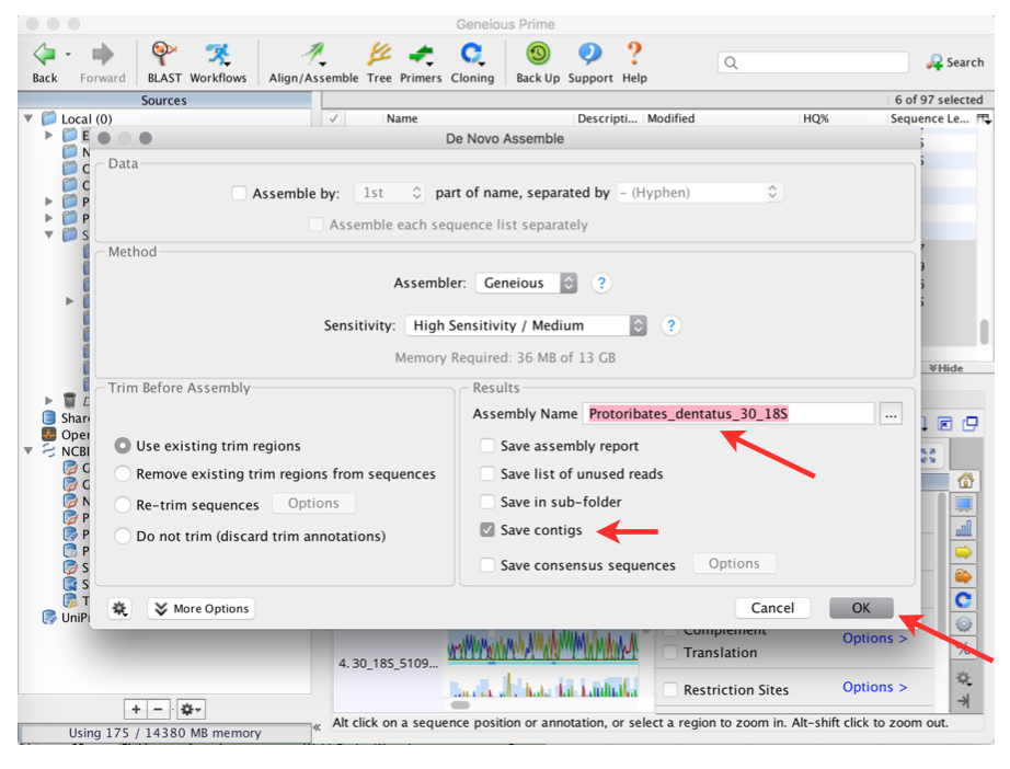
Select De Novo Assemble from the Align/Assemble menu
(also: Tools —> Align/Assemble —> De Novo Assemble
Provide a name for the newly assembled sequence file
Attention
Never ever use special characters or spaces!
Now all single sequence files are pieced together (=assembled) and all complementary positions of all forward and reverse sequences are displayed underneath each other:
You now have a
.contigfile (not a Sanger file or single nucleotide sequence), which is indicated by the icon in front of the nameScan the contig by eye to ensure that no ambiguous base calls are included
Geneious Prime automatically removes positions (base pairs) at the start/end of each sequence with a quality below a certain quality threshold (, which can be adjusted, if necessary)
Positions that have been removed are indicated by a light pink bar underneath the respective sequence in the chromatogram
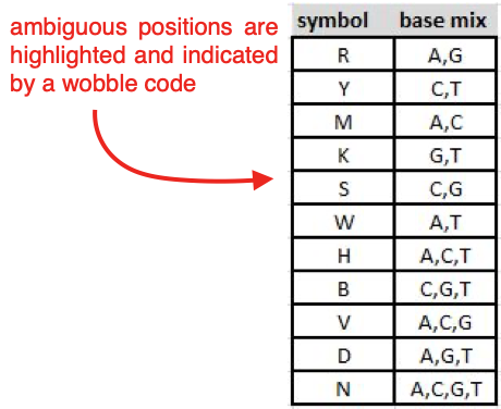
If you have ambiguous positions (indicated by letters that are not
A,C,G, orT; highlighted in red), correct them manually according to the peak call of the sequence with the highest quality at this position.
Note
Correcting the consensus sequence saves the change in both forward and reverse sequence
Correcting the base in the erroneous sequence (either forward or reverse) changes the consensus sequence, but saves the change only in the respective sequence
Note
The table below summarises the symbols used for ambiguous base calls.
After checking and correcting you sequences, export the consensus sequence (= a single sequence that is the combined product of all single sequences)
To export the consensus, see Export Data
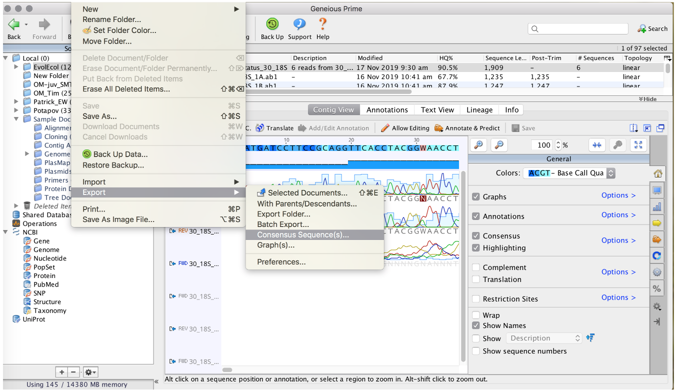
Export Data
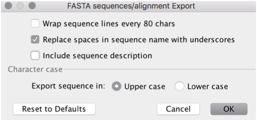
Use the default settings
Threshold: Highest Quality
Assign Quality: Total
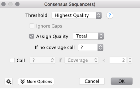
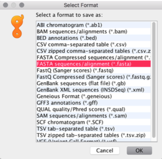
Select Format:
FASTA sequences/alignment (
.fasta)
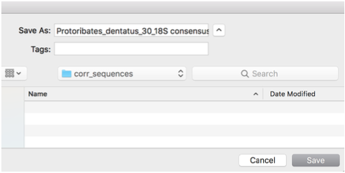
Choose the destination
Again, use default settings
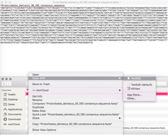
Now you can open the
.fastafile in
Any text editor like Editor or Notepad++ (Windows), TextEdit (Mac), Notepadqq (Linux)
Or in a sequence editor like BioEdit (Windows), AliView (Mac)
Or in Geneious Prime
Database and Search Strategies
Molecular sequence data is available from several online public databases, e.g. NCBI GenBank (USA), EMBL EBI (Europe), or DDBJ (Japan), to name a few. Providers manage and update entries daily via the World Wide Web. During this course, we use the service of NCBI GenBank to compare and validate our own sequence data and obtain additional sequences.
To screen the database for sequence data, two alternative search strategies are described below:
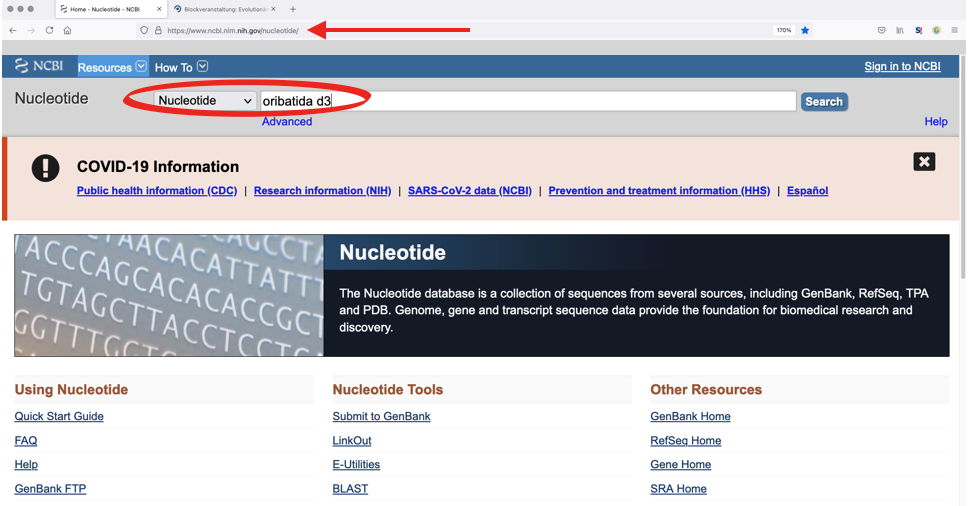
1. Search the database for specific genes and taxa
Enter a species or higher taxon name in the search box. The order of search terms (e.g. ‘oribatida d3’) is neglible, as is the case sensitivity. However, it is important to limit the search to the required database, e.g., ‘Nucleotide’ or ‘Protein’.
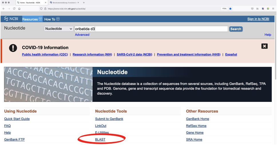
2. BLAST Search
Search for homologous genes using your own sequences.
Note
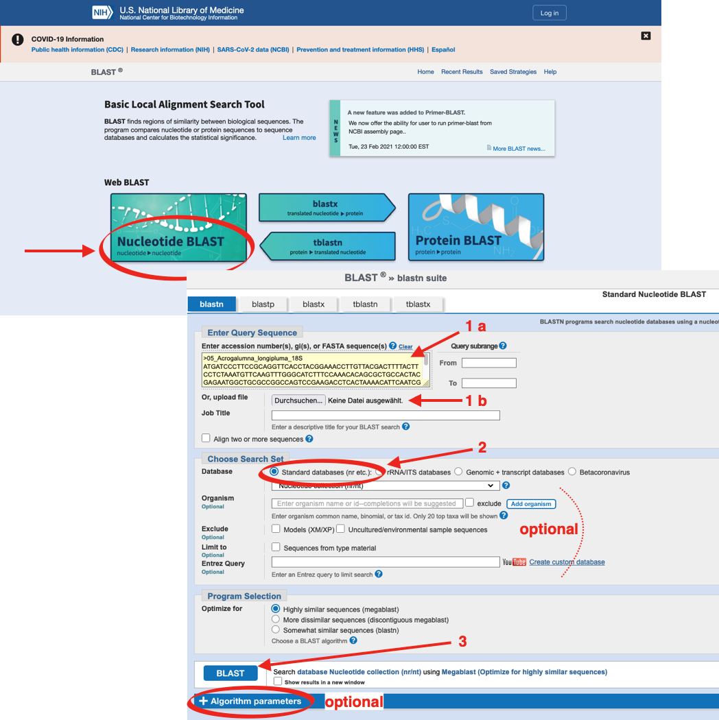
Again, it is important to limit the search to the required database within NCBI, e.g. ‘Nucleotide’ or ‘Protein’.
You can upload your own sequences to the search mask (see below) either by copy-paste (1a) from a sequence editor like BioEdit or MEGA, or sequence files can be uploaded from a directory located on the hard drive (1b). The BLAST search can be accelerated by limiting the search to an appropriate DATABASE (2, mandatory) and to a certain ORGANISM (optional). The search starts when pressing the „BLAST“-button (3).
Tip
The accuracy of search parameters can be adjusted (Algorithm parameters; optional), which affects the degree of similarity of sequences from the database with your sequence data. Downscaling of search parameters can be helpful for searches within variable gene regions or among distantly related (or fast mutating) organisms. Upscaling of search parameters is reasonable when working with repetitive sequences.
After starting a BLAST search a new window will open confirming the search request. The search is finished when a list with all results appears.
Note
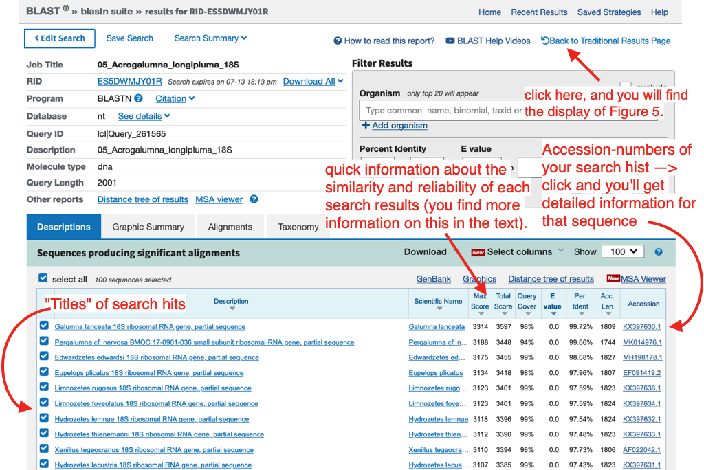
When you click ‘Back to Traditional Results Page’ you will see a graphic that shows how your DNA fragment matches (aligns) with the BLAST results (see below). The graphic represents the complete length of the entered sequence, matching sequences from GenBank are listed below. The colour code illustrates the degree of similarity across the complete sequence and the mouse-over option enables quick assessment of results. When moving the mouse over the graph, names and genes of GenBank entries appear.
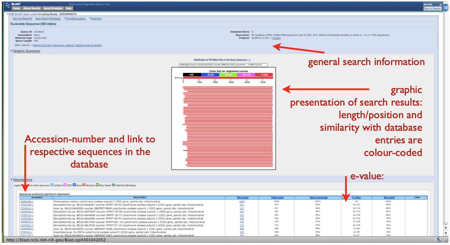
In both figures, detailed results are listed below the graph, providing the accession numbers if the BLAST hits in the last (see above) or first column (see below), linking to the complete database entry with a full description of the sequence. Columns to the right provide information on the degree of similarity and the probability of stochastic agreement. The e-value is the most important, indicating the probability that a database entry matches with the original sequence simply by chance. The smaller the e-value the better: the lower the probability that two sequences match by chance the higher the probability to have a real homologous sequence. Ideally the e-value should be very small (e.g. 2e-152).
Hint
Any published sequence in GenBank is linked with a unique accession number. A GenBank record provides information on the length, name of the gene, and a detailed taxonomic description of the organism from which the sequence derived. Additionally, information on authors and a reference to the publication in which the sequence was first cited are provided within the record, as well as many other things.
Any sequence from GenBank can be downloaded to a local hard drive. The GenBank file format is rather inconvenient and not recognized by some text editors and phylogenetic programs. The most common sequence format supported is FASTA.
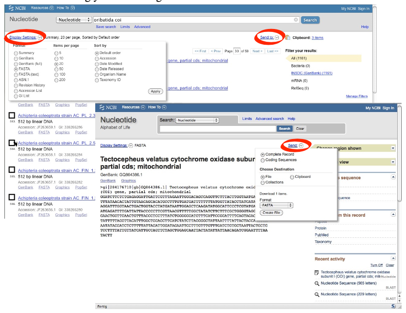
Downloading and Saving
Sequences can be visualized and downloaded in different formats by selecting „Display Settings“ options (top left). Selecting FASTA, the website is updated showing the sequence in the respective file format. To download the sequence on the local hard drive, click on „Send to“ (top right) which opens a drop-down menu to select the destination and format of the sequence file.
Note
Sequences can be saved separately (one-by-one) or as sequence stack (=multiple FASTA file), see below for more.
1. Separate download of sequences from a list of search hits:
Tick the box left to the sequence you wish to save
Go to ‘Send to’ (top right)
Select ‘Complete Record’ (only visible for coding sequences)
‘Choose Destination: File’
‘Download 1 items: Format: FASTA’
Select ‘Create File’, which saves the sequence to your hard drive
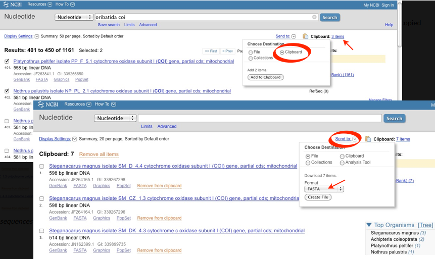
2. Download a stack of sequences from a list of search hits:
Tick all sequences of interest
Go to „Send to“and select „Clipboard“ [files from alternative searches can be added (tick the box left to the sequence → ‘Send to’ → ‘Clipboard’)]
Once all required sequences are saved to the clipboard:
Click on ‘Clipboard’ (top right) and check if your desired sequences are included
Saving the content of the clipboard to a local hard drive:
Go to ‘Send to’ (top right)
Select ‘Complete Record’
‘Choose Destination: File’
‘Format: FASTA’
Select: ‘Create File’, which saves the sequence file to a local hard drive
Note
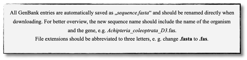
All sequences from the clipboard are now saved in a single file. Remember to change the file name from the default name (=sequences.fasta) to favouritename_favouritegene.fas.
Tip
The Clipboard is a nice and easy way to collect and save large datasets from GenBank. However, if some sequences will be used in different datasets, they must be copied subsequently and saved separately.
Hint
If you wish to download many sequences with continous accession numbers (e.g. from a publication), just enter the first and the last accession number separated by a colon : followed by the tag [accn] or use NCBI’s Batch Entrez.
EF091418:EF091227[accn]
Sequence Editing
Note
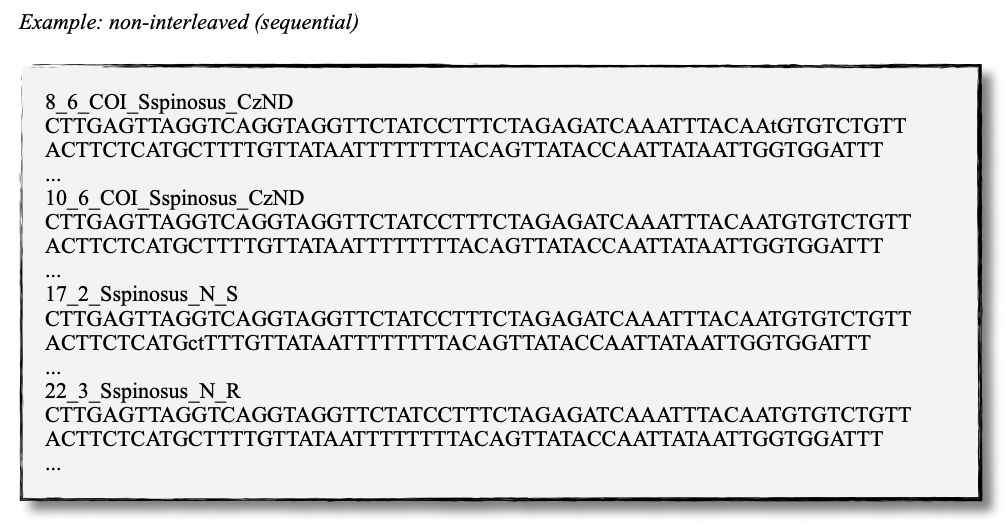
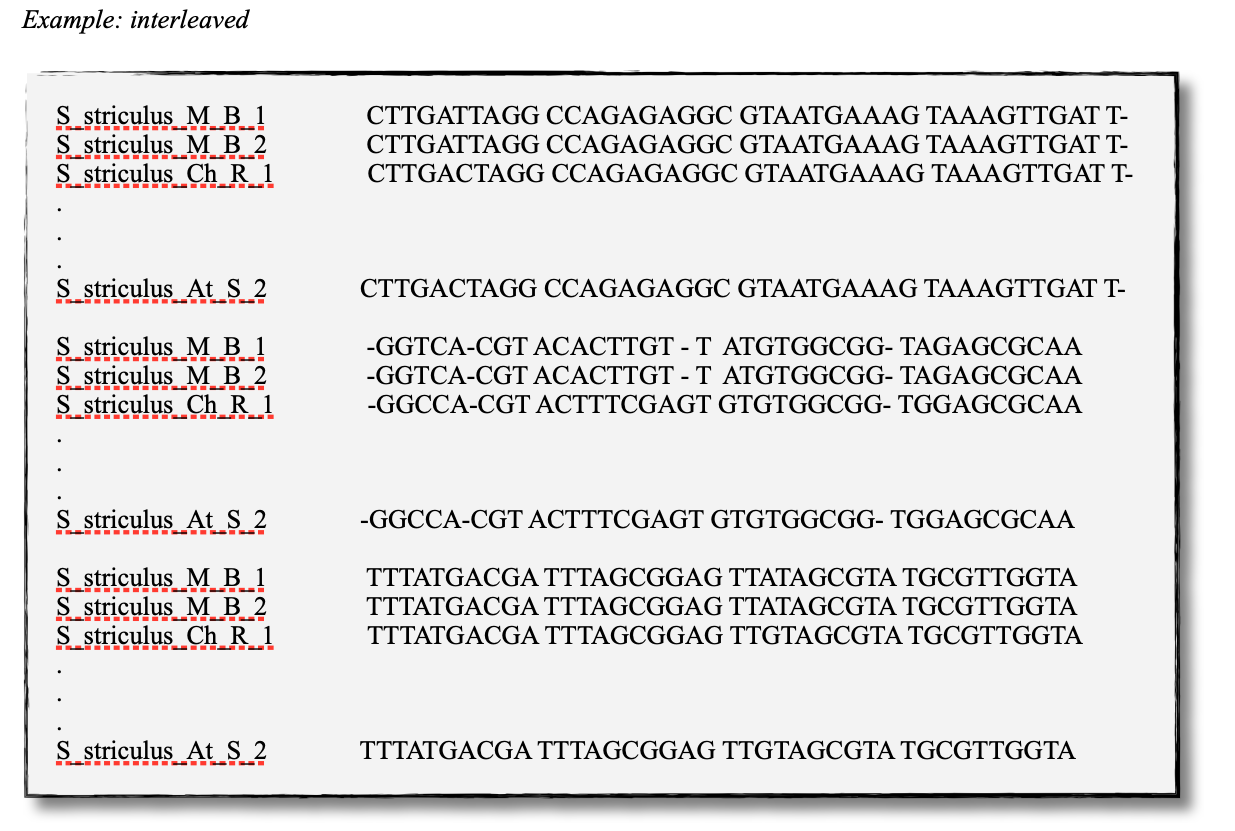
Essentially, sequence data (protein and nucleotide sequences, alignments, etc.) are simple text files. They are edited in a specific format which is recognized by sequence editors and phylogenetic programs. Unfortunately, almost as many formatting styles as analyzing programs exist. Some of the most common editing styles (fasta and text for sequences, phylip and nexus for alignments) are listed here:
Sequence files
Example fasta file ( .fas )
>Archegozetes_longisetosus_COI
GGATCTTCACTG.....
>Atropacarus_sp_COI
GGAACTTCGTTA......
Example txt file ( .txt )
Archegozetes_longisetosus_COI   GGATCTTCACTG....
Atropacarus_sp_COI   GGAACTTCGTTA.....
Alignment files
Example phylip file ( .phy )
2 565
Archegozet   GGATCTTCACT....
Atropacaru   GGAACTTCGTTA...
Example nexus file ( .nex )
#NEXUS
BEGIN DATA;
dimensions ntax=4 nchar=565; format missing=?
interleave=no datatype=DNA gap= -;

matrix
Archegozetes_longisetosus_COI GGATCTTCACTGAGAGCTCTAATCCGTCTCGAATTAGGACAACCAGG...
Hermannia_gibba_COI GGGTCCTCCTTAAGAGGTTTAATTCGACTGGAGTTAGGCCAGCCTGG...
Tectocepheus_velatus_COI GGATCTTCTCTGAGAGGATTGATTCGTTTAGAATTGGGACAGCCAGG...
Atropacarus_sp_COI GGAACTTCGTTAAGGTCTATGATTCGATTTGGGGGGGTTAGGTTCGA...

Models of Sequence Evolution
jModelTest 2 (Darriba et al. 2012)
Compares models of sequence evolution and finds the model that fits best to the dataset
GUI and command line mode
Strategies for statistical model selection include:
Sequential likelihood ratio tests (LRTs)
Akaike Information Criterion (AIC)
Bayesian Information Criterion (BIC)
Performance-based decision theory (DT)
How to compute likelihoods of models of sequence evolution
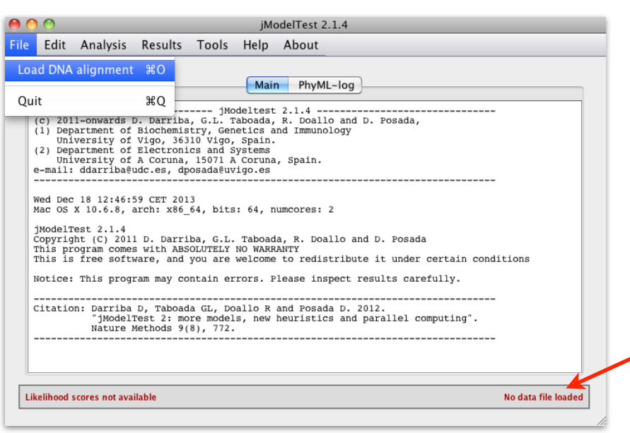
Start the jModelTest GUI (graphical user interface) (for Windows Users: you may double click on the file runjmodeltest-gui.bat sitting in your jmodeltest directory)
java -jar jModelTest.jar
And then load your alignment file into it
File > Load DNA alignment
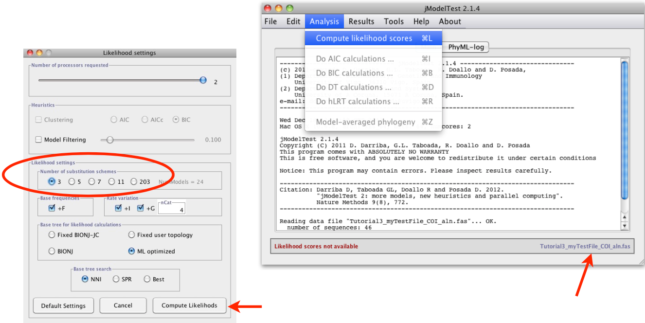
Set up the analysis
Analysis > Compute likelihood scores
Under Likelihood settings choose Number of substitution schemes3
Note
In jModelTest, the number of substitution schemes refers to how many distinct rate matrices are considered when searching for the best-fitting model. It essentially controls how many different ways of grouping the 6 substitution rates are tested. The 6 substitution types (A↔C, A↔G, A↔T, C↔G, C↔T, G↔T) can be grouped into equal or unequal rate classes in different combinations, and each unique grouping defines a different model.
jModelTest offers three options:
3 schemes — tests only the simplest groupings, corresponding to nst=1, nst=2, and nst=6 (i.e., JC/F81, K80/HKY, GTR/SYM)
5 schemes — adds a few intermediate models
11 schemes — tests all possible ways of partitioning the 6 rates, covering 88 models in total
So in short, the more schemes you select, the more thorough the model search — but also the longer it takes. For most purposes, 11 schemes is recommended to ensure the best model is not missed.
Finally, start the analysis with clicking on Compute Likelihoods
After likelihoods have been calculated for each model, a list with all models, parameters and likelihood scores is available under
Results > Show results table
Comparing likelihoods using AIC and BIC
Now we can calculate the model with the best likelihood score. Comparing likelihoods is not easy and sensitive to parameters. In jModelTest different methods (AIC, BIC, DT, and hLRT) are available to estimate the best likelihood.
Attention
Both Akaike Information Criterion (AIC) and Bayesian Information Critierion (BIC) are used in jModelTest to pick the best-fitting substitution model, but they differ in how much they “punish” models for being complex. AIC adds a small penalty for each extra parameter, so it tends to favour more complex models. BIC adds a larger penalty — one that grows with the size of your alignment — so it tends to pick simpler, more conservative models. Because of this, BIC is generally the better choice in phylogenetics, as it is less likely to overfit your data. When both criteria agree on the same model, that’s a good sign. When they disagree, it’s worth checking which models your phylogenetic software actually supports before making a final decision.
In this course, we only want to calculate AIC and BIC (under default settings)
Analysis > Do AIC calculations …
Analysis > Do BIC calculations …
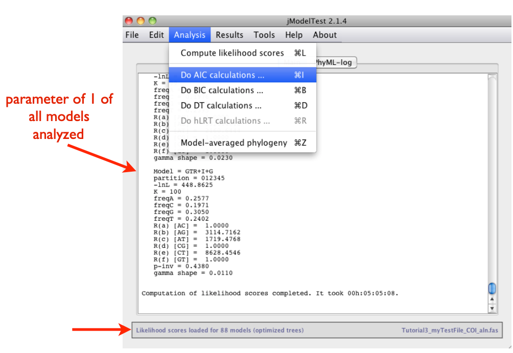
The program provides a very detailed list of the AIC and BIC results. For detailed information on parameters and analyses of jModeltest, click here.
Note
Here’s a quick overview of common models and their nst (number of substitution types) values:
nst = 1 (all substitution rates equal)
JC (Jukes-Cantor)
F81
nst = 2 (transitions and transversions differ)
K80 (Kimura 2-parameter)
HKY85
F84
nst = 6 (all six substitution rates vary)
GTR
SYM
TrN (Tamura-Nei)
TVM
TIM
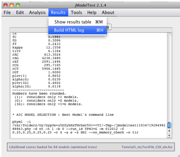
Saving your results
Save your results of AIC and BIC calculations to a HTML log file:
Results > Build HTML log
How to Infer Phylogenetic Trees
Note
Phylogenetic analyses always start with a search for the best tree followed by an a posteriori analysis that statistically checks the probabilities for the tree topology. First, you should get a feeling for properties and logic constraints of phylogenetic trees. For displaying complex trees, use the open source software FigTree.
You will find more information about working with FigTree in the next section How To Draw Phylogenetic Trees.
Neighbor Joining (NJ)
Neighbor Joining is one of the earliest methods to infer phylogenetic trees using molecular data. The method is fast, which makes it attractive for large data sets and for a first analysis to get a „feeling“ for new data sets (Do I need more taxa? Which taxa might be useful? Is the selected outgroup appropriate?), before the longer but more accurate methods Maximum Likelihood (ML) or Bayesian Inference (BI) are used. A disadvantage of this method is that the sequence data cannot be reconstructed from the phylogenetic tree and NJ will not always find the „best“ or the „correct“ tree. The order of taxa in the alignment can also affect the tree topology.
How To Draw Phylogenetic Trees
FigTree (Andrew Rambaut)
This is a versatile program for the graphical visualization of phylogenetic trees. It is recommended to save the opened tree (e.g. the .tre file) directly under a new name to avoid to accidentally overwrite the original tree file.
Open a tree file:
‘File’
‘Open’
Select file containing the trees (e.g. .tre)
Note
Always display the tree with increasing node order (STR + U) and save the tree with a new name (‘File’ → ‘Save As’).
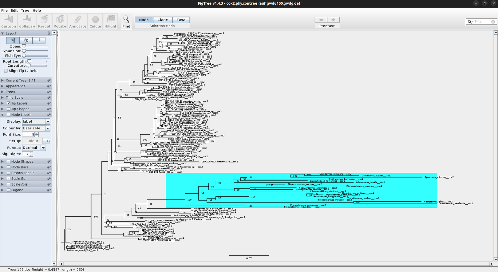
In FigTree, you can make the tree pretty and easy to understand by making lines thicker, increasing font size, and adding colors to branches, clades, or taxa (as shown above). To do this, use the toolbar on the left and top. If you want to annotate or highlight, first assign to either a node, clade, or taxa. Just play around a little bit 🛝. The annotated tree can then be exported as vector graphic, PDF, or bitmap and uploaded in PowerPoint or any other presentation tool.
Attention
All trees in this course should be displayed uniformly. Nodes should spread from the lower left to the upper right side (under ‘Trees’ -> ‘Increasing Node Order’; or STR + U).
The .tre files must be exported (File/Export …) as JPEG in order to import them in PowerPoint or any other presentation tool.
Statistical node support (bootstraps and/or posterior probabilities) are displayed by selecting the tool ‘Node Labels’ or ‘Branch Labels’. These are given as decimals for posterior probabilities (BI) and as percentages for bootstraps (NJ, ML).
In FigTree the relevant results of the phylogenetic analyses can be highlighted or summarized by colouring clades, branches, and tiplabels. In PowerPoint (or in other graphics editors such as Inkscape) you can add annotations, such as boxes, arrows, and other graphical objects.

Maximum Likelihood
Stochastic approach to estimate parameters
Convergence to the „true“ parameters with increasing amount of data
Minimal variation around the „true value“
Calculates a likelihood for each character (any position in an alignment) and requires a lot of computing time
Final tree is calculated from the sum of all likelihoods, the topology with the best (highest) likelihood value is selected
Model of sequence evolution obligatory
RAxML (Randomized Accelerated Maximum Likelihood, Stamatakis 2006)
The ML algorithm in older software (such as PAUP*) is very thorough but even moderately sized datasets (e.g. 40 taxa à 2,000 bp) require days to weeks of computing time. For very large datasets with dozens of genes and hundreds of taxa, a less time-intensive method is necessary. In recent years with advances in high-end computer hardware, new algorithms have been written to improve and accelerate the ML-algorithms used in PAUP*. Meanwhile, several programs exist that calculate Maximum Likelihoods faster than PAUP*. The results of ML analyses can differ between programs even if the same data set and parameters are used. If several programs yield the same results this is further support for the „true“ topology.
RAxML is one of these „fast“ ML-algorithms written for the analysis of large data sets with hundreds of taxa and several genes per taxa. Alignments with 1,900 taxa and 1,200 bp are considered small for RAxML. The high speed for ML analyses is based on the assumption that a topological search (the number of analyzed topologies) is more important for the construction of a „good“ ML tree than the calculation of exact likelihood scores.
Settings in RAxML
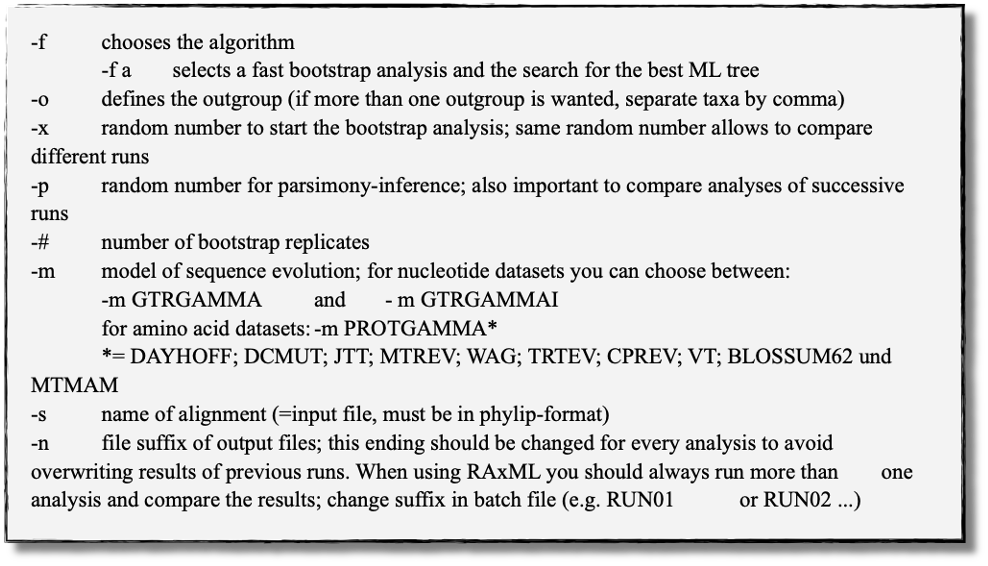
RAxML is not executed via command line or graphical user interface, but with a batch file. The complete command line is written into the batch file before starting the analysis. Here is an example command line for an „easy & fast“ ML analysis with bootstrapping:
RAxML-7.0.3-WIN.exe -f a -o taxaname_1,taxaname_2 -x 12345 -p 12345 -# 500 -m GTRGAMMAI -s name_alignment.phy -n suffix_of_output_file (e.g. Run01)
Start RAxML
Important
The executable file (RAxML-7.0.3-WIN.exe), the batch file (name.batch) and the .phylip file have to be in the same folder. To start the program click on the batch file.
RAxML results
The „easy & fast“ analysis generates four output files:
RAxML_info.RUN01
Text file with all likelihood-values + time/bootstrap
RAxML_bootstrap.RUN01
Text file with all bootstrap trees
RAxML_bestTree.RUN01
Tree with the best likelihood-value without bootstraps
RAxML_bipartitions.RUN01
Tree with the best Likelihood value + bootstraps
Can be open directly in FigTree
Note
These four files should be copied to a separate folder (RAxML_Bsp_18S or ef) after every analysis to avoid overwriting. To limit the risk of overwriting results, each RAxML analysis can also be started from a separate folder. This folder contains all important files (alignment, analysis specific batch file, results) after the analysis.
Bayesian Inference
Maximum Likelihood calculates the probability of your data from which the „best“ tree is inferred. The Bayesian Inference however uses a completely different mathematical approach, the so called posterior probabilities. The assumption is based on the idea that the probability of a hypothesis (the tree) depends on the data (the alignment). For this, prior probabilities (an a priori probability) are assigned to the hypothesis. For each possible tree, specific likelihoods will be calculated based on the data. The hypothesis will be consecutively modified until the „best“ tree is generated to describe the present data. In this way you obtain the probability for a specific hypothesis that is „true“ in the light of a specific dataset. This is the so called posterior probability of the hypothesis.
The hypothesis (the tree) is composed of the three following parameter: topology, branch length and substitution rate. With Bayesian Inference you obtain the „true“ tree if you calculate all possible trees. For this, these three parameters will be adjusted until you obtain a tree that „truely“ describes the data. The number of possible trees is finite, but depending on the size of your dataset it is usually very large. In principle it is possible to find the „true“ tree of the present dataset, but this would take too much time. The challenge for this method is to cleverly draw random samples of all possible trees so that the probability of finding the „true“ tree is high. To investigate the „probability-landscape of the hypothesis“ as effectively as possible the MCMCMC-algorithm (Metropolis-coupled-Marcov-Chain-Monte-Carlo or MC3) has been developed.
MrBayes (Huelsenbeck and Ronquist, 2001)
MrBayes requires an alignment in NEXUS format and can be executed with a batch file or via command line. Parameters are set prior to the analysis and are separated into three parts:
lset (likelihood settings)
prset (prior settings)
mcmc (settings of the MCMC chain)
Before Starting MrBayes
Check whether the alignment file is compatible with MrBayes, it must be in NEXUS format, if necessary change the header manually.
The header for MrBayes should include the following parameter:
#NEXUS
begin data;
dimensions ntax=12 nchar=898;
format datatype=dna interleave=yes gap=-;
matrix
Taxon_1
ACTGTGCTAGTGGGTTACGCTAGCC .....
end;
Tip
Move your alignment in NEXUS format and the executable file of MrBayes (MrBayes.exe for Windows users) to the same folder. This is not mandatory, but otherwise you will have to type in the absolute path of your alignment file which can be tedious.
Parameter Settings and Help
Excute MrBayes
double-click on MrBayes.exe
MrBayes > log start filename=`Gen_name_logfile` (creates log file)

MrBayes > execute `Your_alignment.nex` (load your alignment file)

MrBayes > outgroup `taxon_name` or `outgroup number` (sets the outgroup; you can use the taxon name from your alignment file or its number within the alignment; as default MrBayes recognizes the first taxon of an alignment as outgroup)

MrBayes > help [setting] (detailed explanation of the commands and parameters; it also shows the current settings, for example
MrBayes > help=lset (shows likelihood setting)
MrBayes > help=prset (shows prior setting)
MrBayes > help=mcmc (shows Markov Chain Monte Carlo setting)
Defining the Model of Sequence Evolution
MrBayes > lset nst=1 / 2 / 6 (selects the category of the model of sequence evolution)
               nst=1 (JC/F81)
               nst=2 (K80/HKY85)
               nst=6 (GTR)

MrBayes > lset rates=gamma (model + G = includes Gamma-distribution of substitutions)

MrBayes > lset rates=invgamma (model +I+G = includes both Gamma-distribution and invariant positions)
Note
With the nst element of the lset command, we can specify the JC69 or F81 models (nst=1), the K2P or HKY models (nst=2), or the GTR model (nst=6). You may also check the lecture about Models of Sequence Evolution again.
Setting Priors
You change prior settings with the command prset followed by the parameter. All parameters available for prset are listed when you type help prset.
Note
The default settings of the priors work very well for most analyses.
Here are some of the most important parameters listed:
showmodel (default = flat priors)
for nst=6 (6 parameters possible)
topology (topologypr)
branch-lengths (brlenspr)
frequency of nucleotides (statfreqpr)
6 substitutions of nucleotides (revmatpr)
proportion of invariant positions (pinvarpr)
shape of gamma distributiona (shapepr)
Starting the Analysis
MrBayes > mcmc (starts analysis)
Note
If you do not wish to use the default settings, the following settings must be changed before starting the analysis:
MrBayes > ngen= (number of generations; min. 1x10⁶ - default setting)
MrBayes > nruns= (number of parallel analyses; default settings are 2 independent runs)
MrBayes > nchains= (number of chains: always n-1 hot chains; default setting is 4 (3 cold and 1 heated chain))
MrBayes > samplefreq= (number of generations of a single run; saved to hard drive (default setting: every 500th generation))
MrBayes > printfreq= (number of generations that are printed to the console; default is every 1000th generation)

MrBayes > mcmcp ngen=# nruns=# (using `mcmcp` you can change all parameters without starting the analysis; with `help mcmc` you can check if your changes were saved correctly)
Stopping or Pausing the Analysis
STRG + C+y(stops the run)n(resumes the run)
Writing a batch file (optional)
Open a new file in a text editor (e.g. Notepad++) to write a MrBayes block and save it as .nex file. The batch file must start with the following commands:
#Nexus
begin mrbayes;
enter all commands here, separated by ;
end;
Posterior Analysis
Results for all parameters that were investigated are saved in the files
name.run1.p(for run 1) andname.run2.p(for the parallel run 2)Topologies and branch lengths are saved to the files
name.run1.tandname.run2.t
Important
Average standard deviation of split frequencies should be <0.01 at the end of the analysis, if not you should continue the analysis with more generations!
MrBayes > sump (summarizes the distribution of likelihoods for all saved parameters)
MrBayes > sumt (summarizes the distribution of likelihoods for all saved tree topologies)
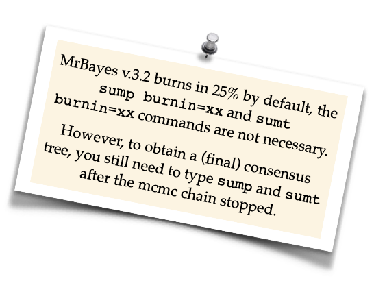
MrBayes > burnin=# (the first # trees must be discarded, because they have low likelihoods compared to the later trees. They should not be incuded in the final analysis as they very likely are very „untrue“ and would corrupt the posterior probabilities)
Note
The burnin should be at least 10% of the sampled trees, 25% is also a common value for burnin. If you were running a chain with 1,000,000 generations with a sample-frequency of 100 (every 100th generation was saved) the command to discard 10% would be: burnin=1000.
It has to be defined after sump (for parameters) and after sumt (for tree topologies), while the burnin values should be identical for both.
MrBayes > sump burnin=#
MrBayes > sumt burnin=#
MrBayes Results
With default paramters MrBayes writes eight output files:
.con(contains the consensus-tree; two trees are written inNewickformat; one tree with and on tree without posterior probabilities. This file can be directly executed in FigTree (see section How To Draw Phylogenetic Trees).
Seven output files document the parameters and their changes during the mcmc analysis:
In separate files for each of the parallel runs (run1 and run2) are all likelihoods of the parameters (
.pfile) and the trees (.tfile) saved that were sampled during the mcmc analyses..trprobscontains all trees and their posterior probabilities that were analysed.partscontains the partition of taxa for the consensus tree and the respective statistics.mcmccontains the parameters of the mcmc-analysis
Ape package
A very short introduction in the Ape package
This tutorial provides basic commands for basic phylogenetic analyses in R. The advantages of using R are that different analyses can be done with one software. Phylogenetic, i.e. sequence data, and ecological data like traits, abundances, and other data like sampling sites, sampling year, can be combined easily.
In the previous tutorials you learned that one program comes for each fundamental analysis, and often files need to be converted when switching between softwares. This can be tedious for phylogenetic analyses and becomes even more complicated and time consuming for phylogenographic and populations genetic analyses, as these often use additional, non-genetic, data to analyses genetic patterns.
Note
The advantages of R seem to be obvious, but one disadvantage is that you need to learn „its language“.
In this tutorial and in this course we provide commands and functions for some basic analyses and to plot the trees. Functions are not explained and we do not introduce you to the syntax of R. However, by playing around and just getting started you can learn already the basics. If you like R and appreciate its potential when it comes to data analysis, you should consider to take different courses, read some books and consult some of the many online tutorials.
Tip
If you feel very insecure about R, check out this online tutorial. It provides a very clear introduction into the basic terminologies and functions of R. On Youtube, you can find many more tutorials on R and RStudio and how to use them to do statistics, phylogenetics, and so on.
Attention
Despite its many advantages, R does not have the stophisticated algorithms and efficiency of a ‘real’ phylogenetic software. When considering publishing your results, you should use the proper software designed for Maximum Likelihood and Bayesian Inference. The ‘proper’ trees can easily be imported into R and used for further analyses.
Getting Started with R
R or RStudio
This is up to you. RStudio is very handy, in particular if you are not used to work in the console. However, the more you get used to R the switch to the command line version of R is not unlikely. In the course you can choose what you like best.
All instructions are given for the console (if not specifically indicated otherwise) but some commands are executed by mouse click in RStudio or even in R, which is not always indicated.
Tip
Make notes in this tutorial which way you prefer or if you find functions you like better than others - you will need all of this again when analyzing your own data later in this course.
Note
# This is an example R code block
> # indicates commands, do not type it
# Expected output is shown in grey
# Comments and notes written after # are ignored by R and shown in green
# Pay attention to quotes ( " " ) in commands, they indicate character strings that can be a vector or a file name or an option within a function
Try to use autocomplete options when working in the console, e.g.
Use the Tab key ↹ when typing a path
Select the pop-up suggestions when typing commands
Use the ↑ arrow key to see previous commands
Attention
If a command did not work, R returns an error message in the console. Always read the error message, most of the time these messages will be helpful and tell you about spelling mistakes or a missing bracket or that it could not find a file because it is not present in your working directory. Regardless, do not hesitate to ask any of the tutors or your neighbour.
Note
The Rscript and all related files can be found here.
Before you import your data:
#Check your working directory
> getwd()
[1] "C:/Users/Desktop/R/"

# Change your working directory to the folder Tutorial 5:
> setwd("C:/Users/Desktop/R/tutorial")
… or in RStudio
To change the working directory just for this sesssion
‘Session’ → ‘Set Working Directory’ → ‘Choose Directory → Browse and select
To set up a working directory as default
‘Tools’ → ‘Global Options’ … → Set default directory (browse and select)
Some useful commands
# lists files in the current working directory
> list.files("C:/Users/Desktop/R/tutorial") # or
> list.files( )
[1] "alnTest_trimmed.fas"      "datafile18S.csv"
[3] "datafile18S.txt"          "my_alignment_aln.fas"
[5] "my18Sphylogeny.tre"       "my28Sphylogeny.tre"
[7] "Onova_example_COI.fas"    "Onova_example_data.csv"
[9] "sequences.fas"            "test.fas"
[11] "Tutorial5_RScript.R"
# gives information about a file
> file.info("18S_Alle.fasta")
                size   isdir          mode     mtime                  ctime
18S_Alle.fasta  27207  FALSE          644      2011-10-13 22:35:48    2016-12-30 22:32:02
                atime                 uid      gid       uname    grname
18S_Alle.fasta  2017-01-04 11:22:04   501      20        hraefn   staff
# lists all objects in current environment
> ls( )
[1]       "countHap"      "countnet"        "dOnova"         "h"       "habitat"
[6]       "HTnet"         "ind.hap"          "list"          "net"
# remove objects, helpful for cleaning up your working environment after playing around with data
> rm(content)  # removes object content, note there will be no warning whatsoever
# returns the class R assigns to objects by R, functions use and require specific classes
> class(my.sequences)
[1] "DNAbin"
# gives internal structure of R object, to some extent useful alternative to summary()
> str(On_data)
'data.frame':      39 obs. of  5 variables:
$ sequence: Factor w/ 39 levels "KF293402_On_HA_F_048",..: 1 2 3 4 5 6 7 8 9 10 ...
$ accn    : Factor w/ 39 levels "KF293402","KF293403",..: 1 2 3 4 5 6 7 8 9 10 ...
$ habitat : Factor w/ 4 levels "F","G","IFG",..: 1 1 1 1 3 3 3 3 4 3 ...
$ site    : Factor w/ 4 levels "HA","KW","SO",..: 1 1 1 1 1 1 1 1 2 2 ...
$ ht      : int  3 3 3 3 4 4 4 4 4 7 …

→ object On_data is a data frame (table) with 39 entries for 5 different variables, these are
•   sequence with 39 different entries, i.e. 39 different sequence names, names are strings (" ")
•   accn with 39 different entries, i.e. 39 different accession numbers, which are are strings (" ")
•   habitat, coded as character (strings = " ") F, G, IFG
•   site, coded as HA, KW, SO
•   ht (= haplotypes in this dataset) which are coded as numbers (integers)
# shows first parts of a vector, matrix, table or data frame; handy to check large datasets
> head(On_data)
                                 sequence       accn      habitat  site   ht
1   KF293402_On_HA_F_048         KF293402       F         HA       3
2   KF293403_On_HA_F_049         KF293403       F         HA       3
3   KF293404_On_HA_F_050         KF293404       F         HA       3
4   KF293405_On_HA_F_051         KF293405       F         HA       3
5   KF293406_On_HA_IFG_053       KF293406       IFG       HA       4
# shows last parts of a vector, matrix, table or data frame; handy to check if (large) dataset is complete
> tail(On_data)
sequence                            accn            habitat              site     ht
34 KF293498_On_UE_IFG_078           KF293498        IFG                  UE       30
35 KF293503_On_UE_IFG_083           KF293503        IFG                  UE       30
36 KF293505_On_UE_IFG_085           KF293505        IFG                  UE       20
37 KF293506_On_UE_IFG_087           KF293506        IFG                  UE       20
38 KF293508_On_UE_IFG_089           KF293508        IFG                  UE       30
39 KF293509_On_UE_IFG_090           KF293509        IFG                  UE
Graphics
> par(mfrow=c(nrow,mcol))   # defines number of rows and columns to graph
> par(mfrow=c(1,2)          # 1 row, 2 columns = 2 graphs next to each other → | |
> par(mfrow=c(2,1)          # 2 rows, 1 column = 2 graphs above each other  → ==
> par(mfrow=c(2,2)          # 2 rows, 2 columns = 4 graphs on one page

> plot( )
> title( "some title")      # adds a title to the first graph
> boxplot(x,main="title")   # boxplot
> hist()                    # histogram
> plot()                    # scatterplot - or phylogenetic tree → plot.phylo( )
Tables
> table <- read.delim( )       # for tab-delimited files (sep="t\")
> table <- read.csv( )         # for comma-delimited files (sep=",")
> table <- read.txt( )         # for space delimited files (sep=" ")
> table                        # returns an object named table, to check that your data was read in correctly
> head( )                      # to check just the first rows
> tail( )                      # to check just the last rows
> table[1,3]                   # gives you the 1st ROW in the third COLUMN in object table
> table[,1,4:10]               # shows you in COLUMN 1 the values of ROWS 4 to 10 in object table
> table[,2,4:10]               # shows you in COLUMN 2 the values of ROWS 4 to 10 in object table
> grep("A",habitat)            # shows you which ROWS have factor A (arable field) in object habitat
> grep("8",site)               # as previous, shows you where you can find site 8 in table
Phylogenetic packages
install.packages("ape")
library(ape)                  # instead of library( ) you can also use require( ), matter of taste
install.packages("pegas")     # install.packages("picante")
library(pegas)                # requires package picante
install.packages("phangorn")
install.packages("seqinr")