Second Week

Major Goals

This week focuses on DNA sequences: how to work with them, where to obtain them if you prefer not to sequence organisms yourself, and how to infer phylogenetic trees.

Lectures and videos provide a step-by-step guide on handling sequence data and conducting phylogenetic analyses. Each day, tutorials will cover a different method, and you must complete each tutorial and its exercises to progress to the next day’s topic.

The week begins with assembling, checking, and exporting your raw sequences (PCR products sequenced last week) to generate high-quality consensus sequences. We start with your DNA sequences to help you become familiar with (1) Sanger DNA sequencing, (2) sequence evaluation (or What’s the difference between a bad and good DNA sequence?), (3) ambiguous (wobble) DNA positions and where do they come from, and (4) DNA sequences derived from public data repositories.

Note

At the end of the week, you will know…

Different kinds of sequence file types.
How to use public databases.
How to edit sequences.
How to check if sequencing results are correct.
What an multiple sequence alignment is.
What a model of sequence evolution is and why it is important for phylogenetic analysis.
What the difference of Cluster algorithms and Search algorithms is when constructing phylogenetic trees.
What ML and BI means.

Monday

Today we will start with recapitulating what you learned last week and discuss the method of Sanger sequencing. After that, you start with processing your sequencing results in Geneious Prime i.e., you will assemble, check and correct the raw reads that have been assigned to you (see sequence assignment list) and export the respective consensus sequences. Then, you can start reading the sections about Geneious Prime and Genbank (see Database and Search Strategies), which introduces you to the handling of sequence data and how to use Genbank, a public sequence data repository.

By doing the exercises in this tutorial, you will generate a toy dataset, which you will be using for the whole week. All following tutorials and exercises are based on this toy dataset.

The basic idea is, that all of you work with the same toy dataset, which makes it easier to compare results. However, it is also fine if you add some of your own sequences (those you checked and exported earlier today).

Tasks of the Day

Read section Geneious Prime and check out the Geneious Prime User Manual.
See the sequence assignment list.
Check out, which raw reads have been assigned to you.

Open Geneious Prime and create the folder Monday/Tutorial_1 and subfolders for each gene.

Local
  ├── Monday
  │     └── Tutorial_1
  │            ├── 18S
  │            ├── 28S
  |            └── COI
  └── …

Download and import your raw sequences to Geneious Prime.

Find the matching raw reads i.e., the forward and the reverse sequence(s) of the same sample (Note that 18S consists of more than two sequences).
Assemble the matching read pairs (Align/Assemble -> De Novo Assemble), store them in separate subfolders (Check the box Save in sub-folder).
Name your consensus sequences in the following format: <Sample number>_<Genus>_<Species>_<Gene>_<Initials> (eg. 1_Acrogalumna_longisetosa_18S_BH).

Local
  ├── Monday
  │     └── Tutorial_1
  │            ├── 18S
  |            |    └── 1_Acrogalumna_longisetosa_18S_BH
  │            ├── 28S
  |            └── COI
  └── …

Check the consensus sequence and correct ambiguous positions.
Export the consensus sequences as FASTA files to your PC.
Upload the consensus files here.

Attention

Never use space or special characters (e.g., ä, ., :) in sequence or file names; always separate words with underscores _. Most sequence editors and phylogenetic programs are very sensitive when it comes to sequence names and file formats. You will save a lot of time, if your file names are compatible right from the start.

For all species from Tutorial 3 (you can find the species names again here), download the 18S rDNA sequences from NCBI GenBank (just as for EF).

Use the Clipboard option to save all sequences in FASTA format as a single file (name the file Tutorial_5_Oribatida_18S.fas).

Attention

There is no 18S rDNA sequence available for Carabodes femoralis, use Carabodes subarcticus. For Platynothrus peltifer, four 18S rDNA sequences are available, download the one with following accession number EF091422 (it’s the longest sequence of the four sequences available).

Hint

A rule of thumb: If two or more sequences are available for a species, always choose the longest sequence.

Take the sequences from Tutorial 3 and copy them to subfolder Tutorial 6.

Local
  ├── Monday
  │     ├── Tutorial_1
  │     └── Tutorial_6
  └── …

Change all sequence names from GenBank to: <GENUS>_<SPECIES>_<ACCESSION NUMBER>_<GENE> (e.g. Archegozetes_longisetosus_EF081321_EF).

Local
  ├── Monday
  │     ├── Tutorial_1
  │     └── Tutorial_6
  │            ├── Archegozetes_longisetosus_EF081321_EF
  │            └── …
  └── …

Open the file Tutorial_5_Oribatida_18S.fas from Tutorial 5 with your local text editor of choice (e.g., Notepad++, Editor).
Change the sequence names from GenBank just as in Tutorial 6 (<GENUS>_<SPECIES>_<ACCESSION NUMBER>_<GENE>).
Import the file to Geneious Prime in a new subfolder Tutorial_7 (as separate sequences).

Local
  ├── Monday
  │     ├── Tutorial_1
  │     ├── Tutorial_5
  │     ├── Tutorial_6
  │     └── Tutorial_7
  │           ├── Archegozetes_longisetosus_EF081321_18S
  │           └── …
  └── …

Note

You now have two datasets with +/- identical taxon sampling but with two different genes. Awesome!

Now you can add (import) some of your own 18S rDNA sequences.
Your own sequences should be named in the same logic as the sequences from NCBI.
Since no accession numbers are available for your sequences, you may replace accession number with own, to quickly identify your own sequences among the others, for example: Archegozetes_longisetosus_own_18S.

Important

Do not add more than four of your own sequences, please. It is helpful to keep the dataset small, because larger datasets will require longer running times (i.e., longer waiting time for you). It will also be more difficult to focus on the most relevant information.

Tip

Just in case, you can read about Geneious Prime again under Sections.

Tuesday

Today, we focus on sequence alignments and their significance in analyzing genetic data. In this tutorial, you will perform sequence alignments using your toy datasets with Geneious Prime.

Remember, sequence files—whether aligned or not—can be saved in various file formats, and the required input format may vary depending on the software you use. If the format is incorrect, the software will not function as expected. Understanding the correct input file format is essential to overcoming initial challenges when working with phylogenetic software.

Note

At the end of the day, you know…

How an alignment is generated by the Needleman-Wunsch algorithm.
How computer algorithms (basically) perform.
The meaning of penalty values and their effects on alignments.
How to find criteria that will help you to decide if an alignment is good or not.
The difference between sequence file formats, and the difference between multifasta and alignment files and how to recognize them.

Important

The different properties of coding and non-coding sequences will not be explained explicitly and we assume that you already know what reading frames are. However, if you are lost, do not hesitate to ask one of the tutors or me.

Tasks of the Day

Read section Alignment.

Note

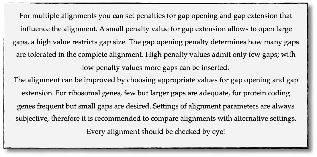
Use your DNA sequences from Monday, namely from Tutorial 6 and Tutorial 7 to generate alignments in Geneious Prime using the parameters below (all other parameters keep in default mode).
In order to do this, mark all sequences in the repective folder and click on Align/Assemble -> Multiple Align -> Geneious Alignment.

Local
  ├── Monday
  │     ├── …
  │     ├── Tutorial_6
  │     |     ├── Archegozetes_longisetosus_EF081321_EF
  │     |     └── …
  │     └── Tutorial_7
  │           ├── Archegozetes_longisetosus_EF081321_18S
  │           └── …
  └── …

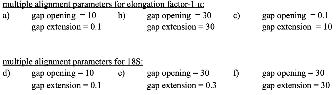
Attention

Use a period . not a comma , when typing the penalty values!

Change the names of the alignments F2 like this 18S_Tutorial_1_a_aln (<GENE>_<TUTORIAL>_<ALIGNMENT LETTER>_aln.) and drag or move them to a new subfolder called Tuesday/Tutorial_1.

Local
  ├── Monday
  └── Tuesday
       └── Tutorial_1
             ├── EF_Tutorial_1_a_aln
             ├── EF_Tutorial_1_b_aln
             ├── EF_Tutorial_1_c_aln
             ├── 18S_Tutorial_1_d_aln
             ├── 18S_Tutorial_1_e_aln
             └── 18S_Tutorial_1_f_aln

Wednesday

Today, we have three learning modules:

Note

By the end of the day, you will:

Understand how phylogenetics accounts for evolutionary changes in DNA sequences, including past changes that are not immediately visible.
Grasp the concept of clustering algorithms, their limitations, and their advantages over search algorithms.
Have constructed four phylogenetic trees using your toy dataset.
Experience the process of a clustering algorithm by manually calculating and drawing a UPGMA tree.
Have practiced drawing phylogenetic trees by hand.

Tasks of the Day

Download and install jmodeltest2 on your PC (you may use this download link directy jmodeltest-2.1.10).
Read section Models of Sequence Evolution.

Read section How to Infer Phylogenetic Trees.
Read section How To Draw Phylogenetic Trees. Don’t be confused—this section primarily focuses on the standalone version of FigTree. However, all the settings explained here are also available in the Geneious Prime plugin.
See also this viewing-and-formatting-trees in Geneious Prime.

Create two subfolders named Wednesday/Tutorial_2/EF and Wednesday/Tutorial_2/18S.

Local
  ├── Monday
  ├── Tuesday
  |    └── Tutorial_1
  └── Wednesday
       └── Tutorial_2
             ├── 18S
             └── EF

Copy your best trimmed alignments from EF and 18S (from Tuesday/Tutorial_1) into their respective subfolders.
For both alignments calculate a NJ tree using the Jukes-Cantor model of sequence evolution (Tree -> Geneious Tree Builder -> Genetic Distance Model: Jukes-Cantor) with 1000 bootstrap replicates (Resample tree -> Resampling Method:Bootstrap + Number of Replicates: 1000).
Root the tree using Zercon sp. (Click on the end of the branch leading to Zercon sp. and hit Root in the subpanel). Why Zercon sp. again?
Indicate in the file name that this tree uses the Jukes-Cantor model, for example, EF_JC_model.

For both alignments calculate a NJ tree using the Tamura-Nei model of sequence evolution and 1000 bootstrap replicates.
Root the tree using Zercon sp.
Indicate in the file name that this tree uses the Tamura-Nei model, for example, EF_TN_model.

Attention

Complete all exercises and questions by hand with pen and paper!
We will discuss them either in the afternoon or tomorrow morning.

Draw the following tree given in Newick Format by hand: ((((A,(B,(C,D))),E),(F,G)),H);.
Check your topology using FigTree in Geneious Prime.

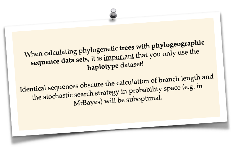
Phylogeography is the study of the genetic structure of species within or between geographic regions. If populations are geographically distant from each other, gene flow is usually reduced and both populations accumulate mutations independently, which increases genetic distance between taxa. If gene flow continues between geographically distant populations, or if they share a common ancestor from which they recently separated, their genetic distance is comparatively small.

Note

In the course of a Master’s thesis, a student investigates the relationships of two populations of the oribatid mite Steganacarus magnus (SM) from Germany (D) and France (F). To understand the relationships between the two populations, the student sequenced the COI mitochondrial gene of seven individuals and generated a matrix that shows the genetic distances between all individuals (see distance matrix under Exercise).

Attention

Do it all by hand with pen and paper!

To infer if the two populations have a recent common ancestor, draw a UPMGA tree and calculate the length of all tree branches.
Write down the tree with all distance calculations and intermediate distance matrixes.
Interpret the tree in a phylogeographic context.
Are both populations genetically separated or are there any indications for gene flow or dispersal?

	SM_D1	SM_D2	SM_D3	SM_D4	_SM_F1	SM_F2
SM_D1
SM_D2	5
SM_D3	6	1
SM_D4	42	39	40
SM_F1	5	2	3	39
SM_F2	67	68	71	70	68
SM_F3	72	73	74	72	73	6

Thursday

Today, it’s all about search algorithms. You will learn the basics of the two most common methods for calculating phylogenetic trees – Maximum Likelihood in the morning and Bayesian Inference in the afternoon.

Both methods are widely used, because they are more thorough than clustering algorithms (such as UPGMA or NJ) and they approach the mathematical part of inferring phylogenetic trees from different angles. You will hear more about this in the Lectures that are accompanied with the two sections.

Both programs can be installed as plugins in Geneious Prime. See Tutorial 1 and Tutorial 2 for doing so.

Note

Both programs can also be controlled via the command line – you may use this approach during the third week to improve the computing performance of both RAxML (download here) and MrBayes (download here).

While working through the exercises, many topics you have been dealing with earlier this week will come up again, such as input file format or Models of Sequence Evolution.

Note

At the end of the day you will…

Know the difference between cluster and search algorithms.
Know why search algorithms take so much longer for analysing genetic data than cluster algorithms.
Know that ML uses likelihoods, and MrBayes uses posterior probabilities.
Know what MCMC is and for which type of analysis it is used.
Be able to interpret the different statistics MrBayes provides.
Understand the meaning of prior and posterior probabilities.
Understand the difference between bootstrap support and posterior probabilites and why they are not directly comparable.

Tasks of the Day

Read section RAxML. Don’t be confused—this section primarily focuses on the command-line version of RAxML. However, all the settings explained here are also available in the Geneious Prime plugin.
Install the RAxML plugin in Geneious Prime Tools -> Plugins -> Available Plugins.

Create two new subfolders for the RAxML analyses of EF and 18S in Geneious Prime.

Local
  ├── Monday
  ├── Tuesday
  ├── Wednesday
  └── Thursday
       └── Tutorial_1
             ├── 18S
             └── EF

Copy your best alignments from EF and 18S (from Tuesday/Tutorial_1) into their respective subfolders.
Start the ML analyses with following parameters Tree -> RAxML:
- GTR GAMMA I Nucleotide Model:GTR GAMMA I
- Rapid bootstrapping and search for best-scoring ML tree Algorithm:Rapid bootstrapping and search for best-scoring ML tree: Command line: -f a -x 1
- 500 bootstrap replicates Number of starting trees or bootstrap replicates:500
- Any other parameter in default settings
Write down how long the analyses took (in seconds).

Read section MrBayes. Don’t be confused—this section primarily focuses on the command-line version of MrBayes. However, all the settings explained here are also available in the Geneious Prime plugin.
Install the MrBayes plugin in Geneious Prime Tools -> Plugins -> Available Plugins.

Create two new subfolders for the MrBayes analyses of EF and 18S in Geneious Prime.

Local
  ├── Monday
  ├── Tuesday
  ├── Wednesday
  └── Thursday
       ├── Tutorial_1
       └── Tutorial_2
             ├── 18S
             └── EF

Copy your best alignments from EF and 18S (from Tuesday/Tutorial_1) into their respective subfolders.
Start the Bayesian Inference using MrBayes Tree -> MrBayes with following parameters:
- Use GTR+G+I as model of sequence evolution Substitution Model:GTR + Rate Variation: invgamma
- Set the outgroup Outgroup: Zercon sp.
- Use 1 million generations Chain Length:1,000,000 and sample every 100th generation Subsampling Freq:100
- Use a burn-in of 10% Burn-in Length:1000
Write down how long the analysis took (minutes + seconds).

Which parameter-settings deviate from the default settings?
What is the Average standard deviation of split frequencies of your analyses? Use EF_Tutorial_1_b_aln - Posterior output and look for the tab Raw Posterior Output in the lower panel. There you will find a column StdDev(s). Click on Show entire ### bytes (may be very slow) to show the whole output.

Note

The Average standard deviation of split frequencies is a measure used in Bayesian phylogenetic inference to assess convergence and stability of the MCMC (Markov Chain Monte Carlo) chains during the analysis. The split frequency measures how often a particular split appears across all sampled trees from an MCMC chain.

< 0.01 — generally accepted as indicating good convergence; the two MCMC runs are sampling from the same distribution

< 0.05 — acceptable for a preliminary analysis, but ideally you should run the chains longer

> 0.05 — indicates the runs have not converged and results should not be trusted; chains need to run longer

Friday

Now you know all the essential steps and methods how to calculate a phylogenetic tree from sequence data. You may have realized that you had to use different file formats for different programs and different programs for different analyses.

You should also know that you can work with sequence data and make phylogenetic trees in R. One big advantage of using R is, that you can do all analyses in one software, without reformatting the input files.

The other big advantage of R is, that you can do awesome downstream analyses with your phylogenetic tree, like analysing trait evolution when you have trait data for your taxa, or analyse community data. But this is another story.

This day is dedicated to introduce you into the basic commands in R that enable you to calculate a phylogenetic tree. Of course: R walks along the analytical path from sequence to tree in its very own way. However, this may even help you to better remember or even understand the single steps that are involved in building a phylogenetic tree from scratch.

Depending on your present day R skills, you may only skim through some of the sections. You will see which are relevant for you to read.

Note

At the end of the day, you will…

Be more versatile and confident when working with genetic data in R.

Tasks of the Day

Read section Ape package.
Read section Getting Started with R.
Install R and RStudio.
Download the R script and the example files here.

Export your sequences from Monday/Tutorial_6 and Monday/Tutorial_7 as FASTA files to your PC. Name them Oribatida_18S.fas and Oribatida_EF.fas, respectively.
Open R or RStudio and set the folder containing the files as the working directory.
Remember to (download and) activate all required packages.

Align the multifasta sequences Oribatida_EF.fas and Oribatida_18S.fas using the msa( ) function in R.
Use the CLUSTAL algorithm and set 10 and 0.1 as gap opening and gap penalties, respectively.
Save the alignments as EF_aln1.fas and 18S_aln1.fas.
Open the alignments in Geneious Prime, check and trim to the shortest sequence.
Export the trimmed alignments as EF_aln2.fas and 18S_aln2.fas to your PC preferably in the same folder as your other files.

Calculate a Neighbor Joining tree based on p-distances for EF_aln2.fas and 18S_aln2.fas.
Save the distance matrix for each alignment as csv, name them distance_EF.csv and distance18S.csv, to your PC.
Calculate 1000 bootstraps for each tree.
Plot each tree neatly (ladders.right = FALSE, cex = 0.7), displaying bootstrap values as percentages in lightblue text color, enclosed by circles with a white background..
Save the NJ trees with nodelabels as JPG: 1) The NJ_EF.tre with red tip labels and 2) the``NJ_18S.tre`` with lightblue tip labels.

Calculate the model of sequence evolution in R for the trimmed alignments EF_aln2.fas and 18S_aln2.fas.

Calculate ML trees for EF_aln2.fas and 18S_aln2.fas, respectively.
Root both trees with the outgroup Zercon.
Plot both trees in one graphic, with facing tip labels. EF with green and 18S with yellowgreen tip labels.
Display bootstrap values enclosed in red circles with a pink1 background.
Save both trees in one plot as PDF to your PC, name it ML_EF_18S.pdf.